The goal here is to practice building convolutional neural networks to classify notMNIST characters using TensorFlow. As image size become bigger and bigger, it become unpractical to train fully-connected NN because there will be just too many parameters and thus the model will overfit very soon. And CNN solve this problem by weight sharing.
We will start by building a CNN with two convolutional layers connected by a fully connected layer and then try also pooling layer and other thing to improve the model performance.
Original jupyter notebook originated from the Udacity MOOC course: Deep learning by Google.
Import libraries
# These are all the modules we'll be using later. Make sure you can import them
# before proceeding further.
from __future__ import print_function
import numpy as np
import seaborn as sns
import tensorflow as tf
import matplotlib.pyplot as plt
from six.moves import cPickle as pickle
from six.moves import range
from tqdm import tnrange
import time

# beautify graph
plt.style.use('ggplot')
Load notMNIST dataset
pickle_file = 'datasets/notMNIST.pickle'

with open(pickle_file, 'rb') as f:
    save = pickle.load(f)
    train_dataset = save['train_dataset']
    train_labels = save['train_labels']
    valid_dataset = save['valid_dataset']
    valid_labels = save['valid_labels']
    test_dataset = save['test_dataset']
    test_labels = save['test_labels']
    del save  # hint to help gc free up memory
    print('Training set', train_dataset.shape, train_labels.shape)
    print('Validation set', valid_dataset.shape, valid_labels.shape)
    print('Test set', test_dataset.shape, test_labels.shape)
Reformat data
Reformat into a TensorFlow-friendly shape:
- convolutions need the image data formatted as a cube of shape (width, height, #channels)
- labels as float 1-hot encodings.
image_size = 28
num_labels = 10
num_channels = 1  # grayscale


def reformat(dataset, labels):
    dataset = dataset.reshape((-1, image_size, image_size,
                               num_channels)).astype(np.float32)
    labels = (np.arange(num_labels) == labels[:, None]).astype(np.float32)
    return dataset, labels


train_dataset, train_labels = reformat(train_dataset, train_labels)
valid_dataset, valid_labels = reformat(valid_dataset, valid_labels)
test_dataset, test_labels = reformat(test_dataset, test_labels)
print('Training set', train_dataset.shape, train_labels.shape)
print('Validation set', valid_dataset.shape, valid_labels.shape)
print('Test set', test_dataset.shape, test_labels.shape)
def accuracy(predictions, labels):
  return (100.0 * np.sum(np.argmax(predictions, 1) == np.argmax(labels, 1))
          / predictions.shape[0])
Helper for training visualization
Let's define a function that make better visualization of our training progress.
The function will draw mini-batch loss and training/validation accuracy dynamically.
# dynamic showing loss and accuracy when training
%matplotlib notebook

def plt_dynamic(x, y, ax, xlim=None, ylim=None, xlabel='X',
                ylabel='Y', colors=['b'], sleep_sec=0, figsize=None):
    import time
    if figsize: fig.set_size_inches(figsize[0], figsize[1], forward=True)
    ax.set_xlabel(xlabel); ax.set_ylabel(ylabel)
    for color in colors: ax.plot(x, y, color)
    if xlim: ax.set_xlim(xlim[0], xlim[1])
    if ylim: ax.set_ylim(ylim[0], ylim[1])

    fig.canvas.draw()
    time.sleep(sleep_sec)
NN with 2 convolutional layers
Let's build a small network with two convolutional layers, followed by one fully connected layer. Convolutional networks are more expensive computationally, so we'll limit its depth and number of fully connected nodes.
Computation graph
Although this assignment already provide good Tensorflow code to build convoluational networks, I found that I can't imagine what NN I was going to build by reading the code. So I tried to draw what we're going to build and explain some parameters used in code by comments.
The convolutional network we're going to build:
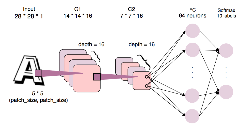
Something worth mentioning:
- We set both convoluational layers' output depth = 16.
- We use filters/patches of shape (5 * 5) to find features in local area of a image.
- The new width and height of the convoluational layer will be half of that in the previous layer because we use stride = 2 and SAME padding to 'slide' our patches. Thus 28 -> 14 -> 7.
- Notice that ReLU layers applied after convoluational layers are omitted for simplicity.
- The activations in C2 fully connected to the FC layer. For each neuron on the FC layer, there are $7 * 7 * 16 = 784$ weights ($785$ for bias ), so there are $785 * 64 = 50240$ parameters in the FC layer.
For more details about CNN, I recommend CS231n.
batch_size = 16
patch_size = 5
depth = 16
num_hidden = 64

graph = tf.Graph()

with graph.as_default():

    # Input data.
    tf_train_dataset = tf.placeholder(
        tf.float32, shape=(batch_size, image_size, image_size, num_channels))
    tf_train_labels = tf.placeholder(
        tf.float32, shape=(batch_size, num_labels))
    tf_valid_dataset = tf.constant(valid_dataset)
    tf_test_dataset = tf.constant(test_dataset)

    # Variables.
    # When defining weights for a convoluational layer, use the notation
    # [filter_size, filter_size, input_depth, output_depth]
    layer1_weights = tf.Variable(
        tf.truncated_normal(
            [patch_size, patch_size, num_channels, depth], stddev=0.1))
    layer1_biases = tf.Variable(tf.zeros([depth]))

    # in this CNN, two convoluational layers happen to have the same depth.
    # if we want, we can adjust them to be different like depth1, depth2
    layer2_weights = tf.Variable(
        tf.truncated_normal(
            [patch_size, patch_size, depth, depth], stddev=0.1))
    layer2_biases = tf.Variable(tf.constant(1.0, shape=[depth]))

    # because we use stride = 2 and SAME padding, our new shape of first feature map C1
    # will be (image_size // 2, image_size //2). and because we use 2 convolutional layers,
    # the shape of second feature map C2 will be (image_size // 2 // 2, image_size // 2 // 2)
    # = (image_size // 4, image_size // 4). and because we have depth == 16,
    # the total neurons on C2 will be image_size // 4 * image_size // 4 * depth
    layer3_weights = tf.Variable(
        tf.truncated_normal(
            [image_size // 4 * image_size // 4 * depth, num_hidden],
            stddev=0.1))
    layer3_biases = tf.Variable(tf.constant(1.0, shape=[num_hidden]))
    layer4_weights = tf.Variable(
        tf.truncated_normal([num_hidden, num_labels], stddev=0.1))
    layer4_biases = tf.Variable(tf.constant(1.0, shape=[num_labels]))

    # Model.
    def model(data):
        # this is where we set stride = 2 for both width and height and also SAME padding
        # the third parameters in tf.nn.conv2d is to set stride for every dimension
        # specified in the first parameter data's shape
        conv = tf.nn.conv2d(data, layer1_weights, [1, 2, 2, 1], padding='SAME')
        hidden = tf.nn.relu(conv + layer1_biases)
        conv = tf.nn.conv2d(
            hidden, layer2_weights, [1, 2, 2, 1], padding='SAME')
        hidden = tf.nn.relu(conv + layer2_biases)
        shape = hidden.get_shape().as_list()

        # turn the C2 3D cube back to 2D matrix by shape (#data_points, #neurons)
        reshape = tf.reshape(hidden,
                             [shape[0], shape[1] * shape[2] * shape[3]])
        hidden = tf.nn.relu(tf.matmul(reshape, layer3_weights) + layer3_biases)
        return tf.matmul(hidden, layer4_weights) + layer4_biases

    # Training computation.
    logits = model(tf_train_dataset)
    loss = tf.reduce_mean(
        tf.nn.softmax_cross_entropy_with_logits(
            labels=tf_train_labels, logits=logits))

    # Optimizer.
    optimizer = tf.train.GradientDescentOptimizer(0.05).minimize(loss)

    # Predictions for the training, validation, and test data.
    train_prediction = tf.nn.softmax(logits)
    valid_prediction = tf.nn.softmax(model(tf_valid_dataset))
    test_prediction = tf.nn.softmax(model(tf_test_dataset))
Train the model and visualize the result
The best thing of the visualization is that it's rendered in a real-time manner.
num_steps = 1001
step_interval = 50


with tf.Session(graph=graph) as session:
    # initialize weights
    tf.global_variables_initializer().run()

    # plot for mini-batch loss and accuracy
    fig, (ax1, ax2, ax3) = plt.subplots(3, 1, sharex=True)
    xs, batch_loss, batch_acc, valid_acc = [[] for _ in range(4)]

    for step in tnrange(num_steps):
        # get new mini-batch for training
        offset = (step * batch_size) % (train_labels.shape[0] - batch_size)
        batch_data = train_dataset[offset:(offset + batch_size), :, :, :]
        batch_labels = train_labels[offset:(offset + batch_size), :]
        feed_dict = {
            tf_train_dataset: batch_data,
            tf_train_labels: batch_labels
        }
        _, l, predictions = session.run(
            [optimizer, loss, train_prediction], feed_dict=feed_dict)


        # draw loss and accuracy while training
        if (step % step_interval == 0):

            xs.append(step)
            batch_loss.append(l)
            batch_acc.append(accuracy(predictions, batch_labels))
            valid_acc.append(accuracy(valid_prediction.eval(), valid_labels))

            plt_dynamic(xs, batch_loss, ax1, (0, num_steps),
                        None, '#Iterations', 'Mini-batch Loss')
            plt_dynamic(xs, batch_acc, ax2, (0, num_steps),
                        (0, 100), '#Iterations', 'Mini-batch Acc')
            plt_dynamic(xs, valid_acc, ax3, (0, num_steps),
                        (0, 100), '#Iterations', 'Valid Acc', colors=['r'], figsize=(7, 7))

            if (step % (step_interval * 2) == 0):

                print('Minibatch loss at step {}: {:.3f}.'.format(step, l) +
                      'batch acc: {:.1f}%, Valid acc: {:.1f}%.'\
                      .format(accuracy(predictions, batch_labels),
                              accuracy(valid_prediction.eval(), valid_labels)))

    print('Test accuracy: %.1f%%' % accuracy(test_prediction.eval(),
                                             test_labels))

As shown above, mini-batch loss dropped rapidly at first 200 iterations, training and validation accuracy also improve quickly (both achieved about 80%). After 200 iterations, validation performance become stable but still improved about 5%. The test accuracy is about 89%.
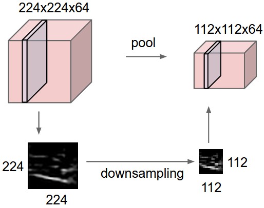
Problem 1 - Use pooling layers to reduce dimensionality
The convolutional model above uses convolutions with stride 2 to reduce the dimensionality. Replace the strides by a max pooling operation (nn.max_pool()) of stride 2 and kernel size 2.
The reason why we're going to use pooling layer is that we can reduce spatial size thus parameters to reduce the chance of overfitting. And the advantage of pooling layer is that it require no new parameters. Let's see how much performance we can gain by using max pooling.
Build model with pooling layers
Actually, what we will do is just to add pooling layers right after ReLU layers and let the convoluational layer use stride 1. In intuition, we let the convoluational layers look more 'closely' into the images, but also try to limit the number of activation and extract the important parts by pooling layers.
batch_size = 16
patch_size = 5
depth = 16
num_hidden = 64

graph = tf.Graph()

with graph.as_default():

    # Input data.
    tf_train_dataset = tf.placeholder(
        tf.float32, shape=(batch_size, image_size, image_size, num_channels))
    tf_train_labels = tf.placeholder(
        tf.float32, shape=(batch_size, num_labels))
    tf_valid_dataset = tf.constant(valid_dataset)
    tf_test_dataset = tf.constant(test_dataset)

    # Variables.
    layer1_weights = tf.Variable(
        tf.truncated_normal(
            [patch_size, patch_size, num_channels, depth], stddev=0.1))
    layer1_biases = tf.Variable(tf.zeros([depth]))
    layer2_weights = tf.Variable(
        tf.truncated_normal(
            [patch_size, patch_size, depth, depth], stddev=0.1))
    layer2_biases = tf.Variable(tf.constant(1.0, shape=[depth]))
    layer3_weights = tf.Variable(
        tf.truncated_normal(
            [image_size // 4 * image_size // 4 * depth, num_hidden],
            stddev=0.1))
    layer3_biases = tf.Variable(tf.constant(1.0, shape=[num_hidden]))
    layer4_weights = tf.Variable(
        tf.truncated_normal([num_hidden, num_labels], stddev=0.1))
    layer4_biases = tf.Variable(tf.constant(1.0, shape=[num_labels]))

    # Model.
    def model(data):
        conv = tf.nn.conv2d(data, layer1_weights, [1, 1, 1, 1], padding='SAME')
        hidden = tf.nn.relu(conv + layer1_biases)
        pool = tf.nn.max_pool(hidden, [1, 2, 2, 1], [1, 2, 2, 1], padding='SAME')
        conv = tf.nn.conv2d(pool, layer2_weights, [1, 1, 1, 1], padding='SAME')
        hidden = tf.nn.relu(conv + layer2_biases)
        pool = tf.nn.max_pool(hidden, [1, 2, 2, 1], [1, 2, 2, 1], padding='SAME')
        shape = pool.get_shape().as_list()
        reshape = tf.reshape(pool,
                             [shape[0], shape[1] * shape[2] * shape[3]])
        hidden = tf.nn.relu(tf.matmul(reshape, layer3_weights) + layer3_biases)
        return tf.matmul(hidden, layer4_weights) + layer4_biases

    # Training computation.
    logits = model(tf_train_dataset)
    loss = tf.reduce_mean(
        tf.nn.softmax_cross_entropy_with_logits(
            labels=tf_train_labels, logits=logits))

    # Optimizer.
    optimizer = tf.train.GradientDescentOptimizer(0.05).minimize(loss)

    # Predictions for the training, validation, and test data.
    train_prediction = tf.nn.softmax(logits)
    valid_prediction = tf.nn.softmax(model(tf_valid_dataset))
    test_prediction = tf.nn.softmax(model(tf_test_dataset))
Train the model
num_steps = 1001
step_interval = 50


with tf.Session(graph=graph) as session:
    # initialize weights
    tf.global_variables_initializer().run()

    # plot for mini-batch loss and accuracy
    fig, (ax1, ax2, ax3) = plt.subplots(3, 1, sharex=True)
    xs, batch_loss, batch_acc, valid_acc = [[] for _ in range(4)]

    for step in tnrange(num_steps):
        # get new mini-batch for training
        offset = (step * batch_size) % (train_labels.shape[0] - batch_size)
        batch_data = train_dataset[offset:(offset + batch_size), :, :, :]
        batch_labels = train_labels[offset:(offset + batch_size), :]
        feed_dict = {
            tf_train_dataset: batch_data,
            tf_train_labels: batch_labels
        }
        _, l, predictions = session.run(
            [optimizer, loss, train_prediction], feed_dict=feed_dict)


        # draw loss and accuracy while training
        if (step % step_interval == 0):

            xs.append(step)
            batch_loss.append(l)
            batch_acc.append(accuracy(predictions, batch_labels))
            valid_acc.append(accuracy(valid_prediction.eval(), valid_labels))

            plt_dynamic(xs, batch_loss, ax1, (0, num_steps),
                        None, '#Iterations', 'Mini-batch Loss')
            plt_dynamic(xs, batch_acc, ax2, (0, num_steps),
                        (0, 100), '#Iterations', 'Mini-batch Acc')
            plt_dynamic(xs, valid_acc, ax3, (0, num_steps),
                        (0, 100), '#Iterations', 'Valid Acc', colors=['r'], figsize=(7, 7))

            if (step % (step_interval * 2) == 0):

                print('Minibatch loss at step {}: {:.3f}.'.format(step, l) +
                      'batch acc: {:.1f}%, Valid acc: {:.1f}%.'\
                      .format(accuracy(predictions, batch_labels),
                              accuracy(valid_prediction.eval(), valid_labels)))

    print('Test accuracy: %.1f%%' % accuracy(test_prediction.eval(),
                                             test_labels))

There is some performance gain in my current iteration between model w/o pooling layer ( about 1.3% ). And it seems that after several iterations, the validation set performance is slightly better with the pooling layers. But it took about 1 minute and 30 seconds to train CNN with pooling layers, and only 30 seconds to train the one without pooling layers. I think it depends on whether you're willing to gain a little more performance by using more time to train the model.
Computation graph
batch_size = 16
patch_size = 5
depth = 16
num_hidden = 64

graph = tf.Graph()

with graph.as_default():

    # Input data.
    tf_train_dataset = tf.placeholder(
        tf.float32, shape=(batch_size, image_size, image_size, num_channels))
    tf_train_labels = tf.placeholder(
        tf.float32, shape=(batch_size, num_labels))
    tf_valid_dataset = tf.constant(valid_dataset)
    tf_test_dataset = tf.constant(test_dataset)

    # Variables.
    layer1_weights = tf.Variable(
        tf.truncated_normal(
            [patch_size, patch_size, num_channels, depth], stddev=0.1))
    layer1_biases = tf.Variable(tf.zeros([depth]))
    layer2_weights = tf.Variable(
        tf.truncated_normal(
            [patch_size, patch_size, depth, depth], stddev=0.1))
    layer2_biases = tf.Variable(tf.constant(1.0, shape=[depth]))
    layer3_weights = tf.Variable(
        tf.truncated_normal(
            [patch_size, patch_size, depth, depth], stddev=0.1))
    layer3_biases = tf.Variable(tf.constant(1.0, shape=[depth]))

    # CONV -> FC
    layer4_weights = tf.Variable(
        tf.truncated_normal(
            [(image_size // 8 + 1) * (image_size // 8 + 1) * depth, num_hidden],
            stddev=0.1))
    layer4_biases = tf.Variable(tf.constant(1.0, shape=[num_hidden]))

    # FC -> output
    layer5_weights = tf.Variable(
        tf.truncated_normal([num_hidden, num_labels], stddev=0.1))
    layer5_biases = tf.Variable(tf.constant(1.0, shape=[num_labels]))

    # Model.
    def model(data):
        # [CONV -> RELU -> POOL] * 3
        conv = tf.nn.conv2d(data, layer1_weights, [1, 1, 1, 1], padding='SAME')
        hidden = tf.nn.relu(conv + layer1_biases)
        pool = tf.nn.max_pool(hidden, [1, 2, 2, 1], [1, 2, 2, 1], padding='SAME')
        conv = tf.nn.conv2d(pool, layer2_weights, [1, 1, 1, 1], padding='SAME')
        hidden = tf.nn.relu(conv + layer2_biases)
        pool = tf.nn.max_pool(hidden, [1,2, 2, 1], [1, 2, 2, 1], padding='SAME')
        conv = tf.nn.conv2d(pool, layer3_weights, [1, 1, 1, 1], padding='SAME')
        hidden = tf.nn.relu(conv + layer3_biases)
        pool = tf.nn.max_pool(hidden, [1, 2, 2, 1], [1, 2, 2, 1], padding='SAME')

        shape = pool.get_shape().as_list()
        reshape = tf.reshape(pool,
                             [shape[0], shape[1] * shape[2] * shape[3]])
        hidden = tf.nn.relu(tf.matmul(reshape, layer4_weights) + layer4_biases)
        return tf.matmul(hidden, layer5_weights) + layer5_biases

    # Training computation.
    logits = model(tf_train_dataset)
    loss = tf.reduce_mean(
        tf.nn.softmax_cross_entropy_with_logits(
            labels=tf_train_labels, logits=logits))

    # Optimizer.
    optimizer = tf.train.GradientDescentOptimizer(0.05).minimize(loss)

    # Predictions for the training, validation, and test data.
    train_prediction = tf.nn.softmax(logits)
    valid_prediction = tf.nn.softmax(model(tf_valid_dataset))
    test_prediction = tf.nn.softmax(model(tf_test_dataset))
Train the model
num_steps = 10001
step_interval = 500


with tf.Session(graph=graph) as session:
    # initialize weights
    tf.global_variables_initializer().run()

    # plot for mini-batch loss and accuracy
    fig, (ax1, ax2, ax3) = plt.subplots(3, 1, sharex=True)
    xs, batch_loss, batch_acc, valid_acc = [[] for _ in range(4)]

    for step in tnrange(num_steps):
        # get new mini-batch for training
        offset = (step * batch_size) % (train_labels.shape[0] - batch_size)
        batch_data = train_dataset[offset:(offset + batch_size), :, :, :]
        batch_labels = train_labels[offset:(offset + batch_size), :]
        feed_dict = {
            tf_train_dataset: batch_data,
            tf_train_labels: batch_labels
        }
        _, l, predictions = session.run(
            [optimizer, loss, train_prediction], feed_dict=feed_dict)


        # draw loss and accuracy while training
        if (step % step_interval == 0):

            xs.append(step)
            batch_loss.append(l)
            batch_acc.append(accuracy(predictions, batch_labels))
            valid_acc.append(accuracy(valid_prediction.eval(), valid_labels))

            plt_dynamic(xs, batch_loss, ax1, (0, num_steps),
                        None, '#Iterations', 'Mini-batch Loss')
            plt_dynamic(xs, batch_acc, ax2, (0, num_steps),
                        (0, 100), '#Iterations', 'Mini-batch Acc')
            plt_dynamic(xs, valid_acc, ax3, (0, num_steps),
                        (0, 100), '#Iterations', 'Valid Acc', colors=['r'], figsize=(7, 7))

            if (step % (step_interval * 2) == 0):

                print('Minibatch loss at step {}: {:.3f}.'.format(step, l) +
                      'batch acc: {:.1f}%, Valid acc: {:.1f}%.'\
                      .format(accuracy(predictions, batch_labels),
                              accuracy(valid_prediction.eval(), valid_labels)))

    print('Test accuracy: %.1f%%' % accuracy(test_prediction.eval(),
                                             test_labels))

By adding a new convoluational layer and train 10x steps, our model's performance can even boost to almost 95%! (though it take about 5 minutes to train on my pc) and I think there are still many things we can tune to make the model better, but I will stop here to move on to sequence model!
跟資料科學相關的最新文章直接送到家。 只要加入訂閱名單,當新文章出爐時, 你將能馬上收到通知