The goal here is to progressively train deeper and more accurate models using TensorFlow. We will first load the notMNIST dataset which we have done data cleaning. For the classification problem, we will first train two logistic regression models use simple gradient descent, stochastic gradient descent (SGD) respectively for optimization to see the difference between these optimizers.

Finally, train a Neural Network with one-hidden layer using ReLU activation units to see whether we can boost our model's performance further.

Previously in 1_notmnist.ipynb, we created a pickle with formatted datasets for training, development and testing on the notMNIST dataset.

This post is modified from the jupyter notebook originated from the Udacity MOOC course: Deep learning by Google.

Import libraries¶

# These are all the modules we'll be using later. Make sure you can import them
# before proceeding further.
from __future__ import print_function
import os
import numpy as np
import tensorflow as tf
from six.moves import cPickle as pickle
from six.moves import range

Load notMNIST dataset¶

This time we will use the dataset which has been normalized and randomized before to omit the data preprocessing step.

Tips:

Release memory after loading big-size dataset using del.

pickle_file = 'datasets/notMNIST.pickle'

with open(pickle_file, 'rb') as f:
    save = pickle.load(f)
    print('Dataset size: {:.1f} MB'.format(os.stat(pickle_file).st_size / 2 ** 20))

    train_dataset = save['train_dataset']
    train_labels = save['train_labels']
    valid_dataset = save['valid_dataset']
    valid_labels = save['valid_labels']
    test_dataset = save['test_dataset']
    test_labels = save['test_labels']
    del save  # hint to help gc free up memory
    print('Training set', train_dataset.shape, train_labels.shape)
    print('Validation set', valid_dataset.shape, valid_labels.shape)
    print('Test set', test_dataset.shape, test_labels.shape)

Dataset size: 658.8 MB
Training set (200000, 28, 28) (200000,)
Validation set (10000, 28, 28) (10000,)
Test set (10000, 28, 28) (10000,)

Reformat data for easier training¶

Reformat both pixels(features) and labels that's more adapted to the models we're going to train:

features(pixels) as a flat matrix with shape = (#total pixels, #instances)

Figure 1: Flattened features

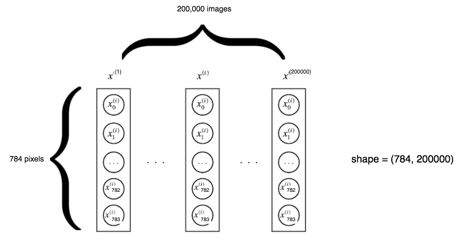
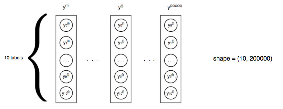
labels as float 1-hot encodings with shape = (#type of labels, #instances)

Figure 2: Flattened labels

Tips:

Notice that we use different shape of matrix with the original TensorFlow example nookbook because I think it's easier to understand how matrix multiplication work by imagining each training/test instance as a column vector. But in response to this change, we have to modify several code in order to make it works!
- Transpose logits and labels when calling tf.nn.softmax_cross_entropy_with_logits
- Set dim = 0 when using tf.nn.softmax
- Set axis = 0 when using np.argmax to compute accuracy
One-hot encode labels by compare the label with the 0-9 array and transform True/False array as float array use astype(np.float32)

image_size = 28
num_labels = 10


def reformat(dataset, labels):
    dataset = dataset.reshape((-1, image_size * image_size)).astype(np.float32).T
    
    # Map 0 to [1.0, 0.0, 0.0 ...], 1 to [0.0, 1.0, 0.0 ...]
    labels = (np.arange(num_labels) == labels[:, None]).astype(np.float32).T # key point1
    return dataset, labels


train_dataset, train_labels = reformat(train_dataset, train_labels)
valid_dataset, valid_labels = reformat(valid_dataset, valid_labels)
test_dataset, test_labels = reformat(test_dataset, test_labels)
print('Training set', train_dataset.shape, train_labels.shape)
print('Validation set', valid_dataset.shape, valid_labels.shape)
print('Test set', test_dataset.shape, test_labels.shape)

Training set (784, 200000) (10, 200000)
Validation set (784, 10000) (10, 10000)
Test set (784, 10000) (10, 10000)

Logistic regression with gradient descent¶

For logistic regression, we use the formula $WX + b = Y'$ to do the computation. W is of shape (10, 784), X is of shape (784, m) and Y' is of shape (10, m) where $m$ is the number of training instances/images. After compute the probabilities of 10 classes stored in Y', we will use built-in tf.nn.softmax_cross_entropy_with_logits to compute cross-entropy between Y' and Y(train_labels) as cost.

We will first instruct Tensorflow how to do all the computation and make it run the optimization several times.

Build the Tensorflow computation graph¶

We're first going to train a multinomial logistic regression using simple gradient descent.

TensorFlow works like this:

First you describe the computation that you want to see performed: what the inputs, the variables, and the operations look like. These get created as nodes over a computation graph. This description is all contained within the block below:
```
with graph.as_default():
    ...
```
Then you can run the operations on this graph as many times as you want by calling session.run(), providing it outputs to fetch from the graph that get returned. This runtime operation is all contained in the block below:
```
with tf.Session(graph=graph) as session:
    ...
```

Let's load all the data into TensorFlow and build the computation graph corresponding to our training:

# With gradient descent training, even this much data is prohibitive.
# Subset the training data for faster turnaround.
train_subset = 10000

graph = tf.Graph()
# when we want to create multiple graphs in the same script,
# use this to encapsulate each graph and run session right after graph definition
with graph.as_default():

    # Input data.
    # Load the training, validation and test data into constants that are
    # attached to the graph.
    tf_train_dataset = tf.constant(train_dataset[:, :train_subset])
    tf_train_labels = tf.constant(train_labels[:, :train_subset])
    tf_valid_dataset = tf.constant(valid_dataset)
    tf_test_dataset = tf.constant(test_dataset)

    # Variables.
    # These are the parameters that we are going to be training. The weight
    # matrix will be initialized using random values following a (truncated)
    # normal distribution. The biases get initialized to zero.
    weights = tf.Variable(
        tf.truncated_normal([num_labels, image_size * image_size]))
    biases = tf.Variable(tf.zeros([num_labels, 1]))

    # Training computation.
    # We multiply the inputs with the weight matrix, and add biases. We compute
    # the softmax and cross-entropy (it's one operation in TensorFlow, because
    # it's very common, and it can be optimized). We take the average of this
    # cross-entropy across all training examples: that's our loss.
    logits = tf.matmul(weights, tf_train_dataset) + biases
    loss = tf.reduce_mean(
        tf.nn.softmax_cross_entropy_with_logits(
            labels=tf.transpose(tf_train_labels), logits=tf.transpose(logits)))

    # Optimizer.
    # We are going to find the minimum of this loss using gradient descent.
    optimizer = tf.train.GradientDescentOptimizer(0.5).minimize(loss)

    # Predictions for the training, validation, and test data.
    # These are not part of training, but merely here so that we can report
    # accuracy figures as we train.
    train_prediction = tf.nn.softmax(logits, dim=0)
    valid_prediction = tf.nn.softmax(
        tf.matmul(weights, tf_valid_dataset) + biases, dim=0)
    test_prediction = tf.nn.softmax(
        tf.matmul(weights, tf_test_dataset) + biases, dim=0)

Tips:

As we saw before, logits = tf.matmul(weights, tf_train_dataset) + biases is equivalent to the logistic regression formula $Y' = WX + b$
Transpose y_hat and y to fit in softmax_cross_entropy_with_logits

Gradient descent by iterating computation graph¶

Now we can tell TensorFlow to run this computation and iterate.
Here we will use tqdm library to help us easily visualize the progress and the time used in the iterations.

Tips:

Use np.argmax(predictions, axis=0) to transfrom one-hot encoded labels back to singe number for every data points.
Use .eval() to get the predictions for test/validation set

from tqdm import tnrange
num_steps = 801


def accuracy(predictions, labels):
    """For every (logit/Z, y) pair, get the (predicted label, label) and count the 
    occurence where predicted label == label and divide by the total number of 
    data points.
    """
    return (np.sum(np.argmax(predictions, axis=0) == np.argmax(labels, axis=0)) 
            / labels.shape[1] * 100)

    # Calculate the correct predictions
#     correct_prediction = tf.equal(tf.argmax(predictions), tf.argmax(labels))

#     # Calculate accuracy on the test set
#     accuracy = tf.reduce_mean(tf.cast(correct_prediction, "float"))
    return accruacy


with tf.Session(graph=graph) as session:
    # This is a one-time operation which ensures the parameters get initialized as
    # we described in the graph: random weights for the matrix, zeros for the
    # biases.
    tf.global_variables_initializer().run()
    print('Initialized')
    for step in tnrange(num_steps):
        # Run the computations. We tell .run() that we want to run the optimizer,
        # and get the loss value and the training predictions returned as numpy
        # arrays.
        _, l, predictions = session.run([optimizer, loss, train_prediction])
        if (step % 100 == 0):
            
            print('Cost at step {}: {:.3f}. Training acc: {:.1f}%, Validation acc: {:.1f}%.'\
                  .format(step, l,
                          accuracy(predictions, train_labels[:, :train_subset]),
                          accuracy(valid_prediction.eval(), valid_labels), ">"))
            
    # Calling .eval() on valid_prediction is basically like calling run(), but
    # just to get that one numpy array. Note that it recomputes all its graph
    # dependencies.
    print('Test acc: {:.1f}%'.format(accuracy(test_prediction.eval(), test_labels)))

Initialized

Cost at step 0: 20.057. Training acc: 6.4%, Validation acc: 10.0%.
Cost at step 100: 2.326. Training acc: 70.9%, Validation acc: 70.7%.
Cost at step 200: 1.868. Training acc: 73.9%, Validation acc: 73.4%.
Cost at step 300: 1.611. Training acc: 75.4%, Validation acc: 74.5%.
Cost at step 400: 1.436. Training acc: 76.4%, Validation acc: 74.8%.
Cost at step 500: 1.306. Training acc: 77.1%, Validation acc: 75.1%.
Cost at step 600: 1.207. Training acc: 77.8%, Validation acc: 75.5%.
Cost at step 700: 1.127. Training acc: 78.5%, Validation acc: 75.6%.
Cost at step 800: 1.062. Training acc: 79.2%, Validation acc: 75.9%.

Test acc: 82.8%

Logistic regression with SGD¶

Or more precisely, mini-batch approach.

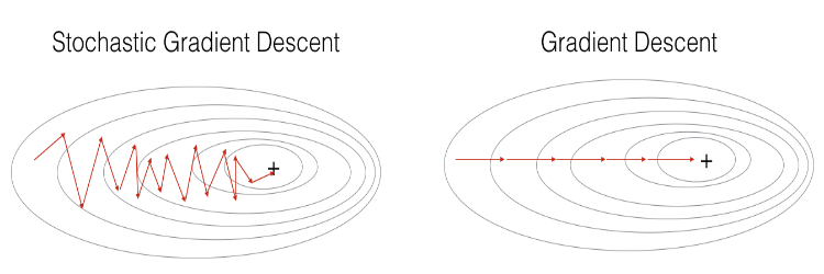
From the result above, we can see it cost about 20 seconds (on my computer) to iterate 10,000 training instances by simple gradient descent. Let's now switch to stochastic gradient descent training instead, which is much faster.

The graph will be similar, except that instead of holding all the training data into a constant node, we create a Placeholder node which will be fed actual data at every call of session.run().

Tips:

The difference between SGD and gradient descent is that the former don't use whole training set to compute gradient descent, instead just use a 'mini-batch' of it and assume the corresponding gradient descent is the way to optimize. So we will keep using GradientDescentOptimizer but with a different loss computed from a smaller sub-training set.

Figure 3: SGD vs Gradient Descent

Build computation graph¶

batch_size = 128

graph = tf.Graph()
with graph.as_default():

    # Input data. For the training data, we use a placeholder that will be fed
    # at run time with a training minibatch.
    tf_train_dataset = tf.placeholder(
        tf.float32, shape=(image_size * image_size, batch_size))
    tf_train_labels = tf.placeholder(
        tf.float32, shape=(num_labels, batch_size))
    tf_valid_dataset = tf.constant(valid_dataset)
    tf_test_dataset = tf.constant(test_dataset)

    # Variables.
    weights = tf.Variable(
        tf.truncated_normal([num_labels, image_size * image_size]))
    biases = tf.Variable(tf.zeros([num_labels, 1]))

    # Training computation.
    logits = tf.matmul(weights, tf_train_dataset) + biases
    loss = tf.reduce_mean(
        tf.nn.softmax_cross_entropy_with_logits(
            labels=tf.transpose(tf_train_labels), logits=tf.transpose(logits)))

    # Optimizer.
    optimizer = tf.train.GradientDescentOptimizer(0.5).minimize(loss)

    # Predictions for the training, validation, and test data.
    train_prediction = tf.nn.softmax(logits, dim=0)
    valid_prediction = tf.nn.softmax(
        tf.matmul(weights, tf_valid_dataset) + biases, dim=0)
    test_prediction = tf.nn.softmax(
        tf.matmul(weights, tf_test_dataset) + biases, dim=0)

Iterate using SGD¶

num_steps = 3001

with tf.Session(graph=graph) as session:
    tf.global_variables_initializer().run()
    print("Initialized")
    for step in tnrange(num_steps):
        # Pick an offset within the training data, which has been randomized.
        # Note: we could use better randomization across epochs.
        offset = (step * batch_size) % (train_labels.shape[1] - batch_size)
        # Generate a minibatch.
        batch_data = train_dataset[:, offset:(offset + batch_size)]
        batch_labels = train_labels[:, offset:(offset + batch_size)]
        # Prepare a dictionary telling the session where to feed the minibatch.
        # The key of the dictionary is the placeholder node of the graph to be fed,
        # and the value is the numpy array to feed to it.
        feed_dict = {
            tf_train_dataset: batch_data,
            tf_train_labels: batch_labels
        }
        _, l, predictions = session.run(
            [optimizer, loss, train_prediction], feed_dict=feed_dict)
        if (step % 500 == 0):
            print('Minibatch loss at step {}: {:.3f}. batch acc: {:.1f}%, Valid acc: {:.1f}%.'\
                  .format(step, l,
                          accuracy(predictions, batch_labels),
                          accuracy(valid_prediction.eval(), valid_labels)))
            
    print('Test acc: {:.1f}%'.format(accuracy(test_prediction.eval(), test_labels)))

Initialized

Minibatch loss at step 0: 20.939. batch acc: 6.2%, Valid acc: 9.7%.
Minibatch loss at step 500: 2.546. batch acc: 70.3%, Valid acc: 75.1%.
Minibatch loss at step 1000: 1.520. batch acc: 74.2%, Valid acc: 76.3%.
Minibatch loss at step 1500: 1.441. batch acc: 76.6%, Valid acc: 77.8%.
Minibatch loss at step 2000: 1.135. batch acc: 79.7%, Valid acc: 77.1%.
Minibatch loss at step 2500: 1.225. batch acc: 72.7%, Valid acc: 78.8%.
Minibatch loss at step 3000: 0.932. batch acc: 76.6%, Valid acc: 79.4%.

Test acc: 86.9%

It took only about 3 seconds in my computer to finish the optimization using SGD (which took gradient descent about 20 seconds) and got a even slightly better result. The key of SGD is take randomized samples / mini-batches and feed that into the model every iteration (thus the feed_dict term).

2-layer NN with ReLU units¶

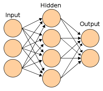
Instead all just linear combination of features, we want to introduce non-linearlity in our logistic regression. By turning the logistic regression example with SGD into a 1-hidden layer neural network with rectified linear units nn.relu() and 1024 hidden nodes, we should be able to improve validation / test accuracy.

A 2-layer NN (1-hidden layer NN) look like this:

Figure 4: 1 hidden-layer NN

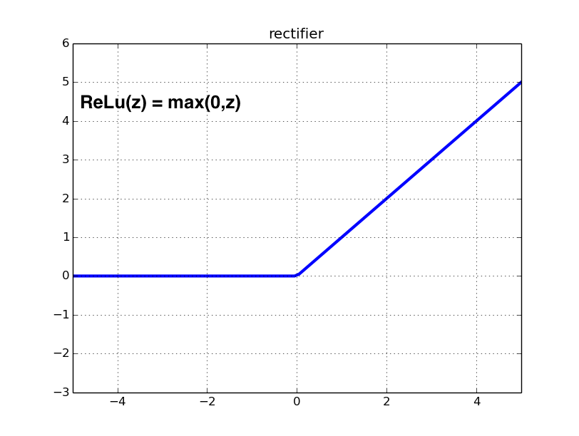
A ReLU activation unit look like this:

Figure 5: ReLU

Build compuation graph¶

In this part, use the notation $X$ in replace of dataset. The weights and biases of the hidden layer are denoted as $W1$ and $b1$, and the weights and biases of the output layer are denoted as $W2$ and $b2$.

Thus the pre-activation output(logits) of output layer is computed as $ logits = W2 * ReLU(W1 * X + b1) + b2 $

batch_size = 128
num_hidden_unit = 1024

graph = tf.Graph()
with graph.as_default():
    # placeholder for mini-batch when training 
    tf_train_dataset = tf.placeholder(
        tf.float32, shape=(image_size * image_size, batch_size))
    tf_train_labels = tf.placeholder(
        tf.float32, shape=(num_labels, batch_size))
    
    # use all valid/test set
    tf_valid_dataset = tf.constant(valid_dataset)
    tf_test_dataset = tf.constant(test_dataset)
    
    # initialize weights, biases
    # notice that we have a new hidden layer so we now have W1, b1, W2, b2
    W1 = tf.Variable(
        tf.truncated_normal([num_hidden_unit, image_size * image_size]))
    b1 = tf.Variable(tf.zeros([num_hidden_unit, 1]))
    W2 = tf.Variable(
        tf.truncated_normal([num_labels, num_hidden_unit]))
    b2 = tf.Variable(tf.zeros([num_labels, 1]))


    # training computation
    logits = tf.matmul(W2, tf.nn.relu(tf.matmul(W1, tf_train_dataset) + b1)) + b2    
    loss = tf.reduce_mean(
        tf.nn.softmax_cross_entropy_with_logits(
            labels=tf.transpose(tf_train_labels), logits=tf.transpose(logits)))
    
    # optimizer
    optimizer = tf.train.GradientDescentOptimizer(0.5).minimize(loss)
    
    # valid / test prediction - y_hat
    train_prediction = tf.nn.softmax(logits, dim=0)
    valid_prediction = tf.nn.softmax(tf.matmul(W2, tf.nn.relu(tf.matmul(W1, tf_valid_dataset) + b1)) + b2, dim=0)
    test_prediction = tf.nn.softmax(tf.matmul(W2, tf.nn.relu(tf.matmul(W1, tf_test_dataset) + b1)) + b2, dim=0)

Run the iterations¶

num_steps = 3001

with tf.Session(graph=graph) as session:
    # initialized parameters
    tf.global_variables_initializer().run()
    
    print("Initialized")
    # take steps to optimize
    for step in tnrange(num_steps):
        
        # generate randomized mini-batches
        offset = (step * batch_size) % (train_labels.shape[1] - batch_size)
        batch_data = train_dataset[:, offset:(offset + batch_size)]
        batch_labels = train_labels[:, offset:(offset + batch_size)]
        
        feed_dict = {
            tf_train_dataset: batch_data,
            tf_train_labels: batch_labels
        }
        
        _, l, predictions = session.run(
            [optimizer, loss, train_prediction], feed_dict=feed_dict)
        
        if (step % 500 == 0):
            print('Minibatch loss at step {}: {:.3f}. batch acc: {:.1f}%, Valid acc: {:.1f}%.'\
                  .format(step, l,
                          accuracy(predictions, batch_labels),
                          accuracy(valid_prediction.eval(), valid_labels)))
            
    print('Test acc: {:.1f}%'.format(accuracy(test_prediction.eval(), test_labels)))

Initialized

Minibatch loss at step 0: 409.203. batch acc: 4.7%, Valid acc: 30.5%.
Minibatch loss at step 500: 12.319. batch acc: 75.8%, Valid acc: 80.7%.
Minibatch loss at step 1000: 12.638. batch acc: 74.2%, Valid acc: 80.8%.
Minibatch loss at step 1500: 7.635. batch acc: 77.3%, Valid acc: 81.2%.
Minibatch loss at step 2000: 7.322. batch acc: 80.5%, Valid acc: 81.4%.
Minibatch loss at step 2500: 10.451. batch acc: 76.6%, Valid acc: 80.1%.
Minibatch loss at step 3000: 3.914. batch acc: 83.6%, Valid acc: 82.7%.

Test acc: 88.7%

Summary¶

Because we use a more complex model(1 hidden-layer NN), it take a little longer to train, but we're able to gain more performance from logistic regression even with the same hyper-parameter settings (learning rate = 0.5, batch_size=128). Better performance may be gained by tuning hyper parameters of the 2 layer NN. Also notice that by using mini-batch / SGD, we can save lots of time training models and even get a better result.

Post Tags Python TensorFlow Deep Learning Neural Networks Optimization NotMNIST Machine Learning Image Recognition SGD Gradient Descent Deep Learning by Google Machine Learning Engineer by kaggle Udacity

Previous Post Regularization for Multi-layer Neural Networks in Tensorflow

Next Post Simple Image Recognition using NotMNIST dataset

View All Post

Using TensorFlow to Train a Shallow NN with Stochastic Gradient Descent

Import libraries¶

Load notMNIST dataset¶

Reformat data for easier training¶

Logistic regression with gradient descent¶

Build the Tensorflow computation graph¶

Gradient descent by iterating computation graph¶

Logistic regression with SGD¶

Build computation graph¶

Iterate using SGD¶

2-layer NN with ReLU units¶

Build compuation graph¶

Run the iterations¶

Summary¶